
LEARNING OUTCOME 8
Graph Data Structure
A graph is a non-linear data structure consisting of nodes (vertices) and edges that connect these nodes. It represents a set of objects (nodes) and the relationships between them (edges). Graphs are used to model various real-world scenarios, such as social networks, transportation networks, and communication networks.
Components of a Graph:
- Vertices (Nodes): These are the fundamental units of a graph. They represent entities or objects.
- Edges: These connect pairs of vertices and represent relationships between them. Edges can be directed or undirected.
Types of Graphs:
- Undirected Graph: Edges have no direction. A connection between two vertices is bidirectional.
- Directed Graph: Edges have a direction. A connection from vertex A to vertex B is different from a connection from B to A.
- Weighted Graph: Edges have associated weights or costs.
- Unweighted Graph: Edges have no associated weights.
- Cyclic Graph: A graph that contains cycles, i.e., paths that start and end at the same vertex.
- Acyclic Graph: A graph that does not contain any cycles.
- Connected Graph: A graph where every vertex is reachable from every other vertex.
- Disconnected Graph: A graph where some vertices are not reachable from others.
Graph Traversals
Graph traversal algorithms are like explorers systematically navigating a complex network of interconnected nodes. They provide a structured approach to visit every reachable node and edge, ensuring no part of the graph is overlooked. This methodical exploration is fundamental for understanding the graph's structure, identifying patterns, and solving problems that involve relationships between nodes, such as finding the shortest path, detecting cycles, or determining connectivity.
Visually a graph traversal is typically drawn as a decision tree, as shown below:
| Traversal Type | Description |
|---|---|
| Depth-First Search (DFS) | Explores as far as possible along each branch before backtracking. |
| Breadth-First Search (BFS) | Explores all neighbors at the present depth prior to moving on to nodes at the next depth level. |
Graph Traversal Issues
- Disconnected Graphs: There may be cases in which the graph is not connected, therefore not all nodes can be reached.
- Cyclic Graphs: In the case of cyclic graphs, we should make sure that cycles do not cause the algorithm to go into an infinite loop.
- Node Re-visitation: We may need to visit some nodes more than once, since we do not know if a node has already been seen, before transitioning to it.
Depth-First Search (DFS)
In this algorithm, we follow one path as far as it will go. The algorithm starts in an arbitrary node, called the root node, and explores as far as possible along each branch before backtracking.
The algorithm can also be applied to directed graphs. DFS is implemented with a recursive algorithm and its temporal complexity is O(E+V).
Conceptual Overview of DFS
The DFS Algorithm starts at the root (top) node of a tree and goes as far as it can down a given branch (path), then backtracks until it finds an unexplored path, and then explores it. The algorithm does this until the entire graph has been explored.
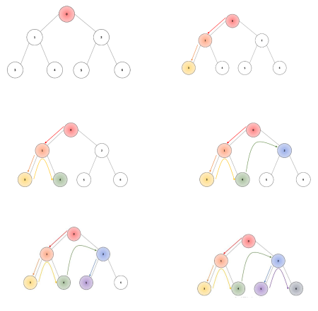
Example of DFS Traversal
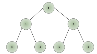
In the example shown below, the root node would be node “0”; we traverse in depth through node “1”, followed by node “3”. Once we reach the node, we move one level up to node “1” and traverse through all other connected nodes, in this case, node “4”. Once we have covered all connected nodes, we move again one level up, to node “0” and traverse all other connected nodes, in this case, node “2”. As we traverse through deeper nodes, we traverse through nodes “5” and “6”, covering all connected nodes.
Breadth-First Search (BFS)
Overview
The BFS algorithm involves pulling out the first element from the queue, checking for a path, and determining if it is the destination node. If not, all children nodes are added to the queue. This process continues by examining all adjacent nodes before moving to the next level.
The algorithm can also be applied to directed graphs. The time complexity is O(E+V).
Conceptual Understanding
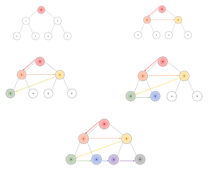
The BFS algorithm begins by searching a start node, followed by its adjacent nodes, and then all nodes reachable by paths containing two edges, three edges, and so forth.
In the example below, the root node is node “0”; we traverse width-wise through node “1”, followed by node “2”. After traversing all nodes in the first depth level, we proceed to the second depth level, starting with node “3”, and moving through nodes “4”, “5”, and “6”.
Example Graph Traversal
Graph Representations
Types of Graph Representations:
- Adjacency List: An Adjacency list is an array consisting of the address of all the linked lists. The first node of the linked list represents the vertex and the remaining lists connected to this node represents the vertices to which this node is connected. This representation can also be used to represent a weighted graph. The linked list can slightly be changed to even store the weight of the edge.
- Adjacency Matrix: Adjacency Matrix is a 2D array of size V x V where V is the number of vertices in a graph. Let the 2D array be adj[][], a slot adj[i][j] = 1 indicates that there is an edge from vertex i to vertex j. Adjacency matrix for undirected graph is always symmetric. Adjacency Matrix is also used to represent weighted graphs. If adj[i][j] = w, then there is an edge from vertex i to vertex j with weight w.
Example Graph:
Let us consider a graph to understand the adjacency list and adjacency matrix representation. Let the undirected graph be:
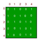
Adjacency Matrix
The adjacency matrix representation of a graph is depicted as follows:
- Definition: In the adjacency matrix representation, a graph is represented in the form of a two-dimensional array.
- Size: The size of the array is V x V, where V is the set of vertices.
The following image represents the adjacency matrix representation:
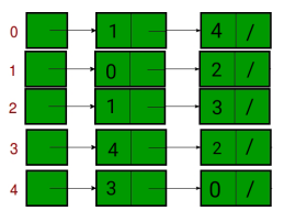
Adjacency List
Definition: In the adjacency list representation, a graph is represented as an array of linked lists. The index of the array represents a vertex and each element in its linked list represents the vertices that form an edge with the vertex.
Visual Representation: The following image represents the adjacency list representation:
Difference Between Adjacency Matrix and Adjacency List
Storage Space:
- Adjacency Matrix: This representation makes use of VxV matrix, so space required in worst case is O(|V|2).
- Adjacency List: In this representation, for every vertex we store its neighbours. In the worst case, if a graph is connected O(V) is required for a vertex and O(E) is required for storing neighbours corresponding to every vertex. Thus, overall space complexity is O(|V| + |E|).
Adding a Vertex:
- Adjacency Matrix: In order to add a new vertex to VxV matrix the storage must be increased to (|V| + 1)2. To achieve this we need to copy the whole matrix. Therefore the complexity is O(|V|2).
- Adjacency List: There are two pointers in adjacency list; the first points to the front node and the other one points to the rear node. Thus, insertion of a vertex can be done directly in O(1) time.
Adding an Edge:
- Adjacency Matrix: To add an edge say from i to j, matrix[i][j] = 1 which requires O(1) time.
- Adjacency List: Similar to insertion of vertex, here also two pointers are used pointing to the rear and front of the list. Thus, an edge can be inserted in O(1) time.
Removing a Vertex:
- Adjacency Matrix: In order to remove a vertex from VxV matrix the storage must be decreased to |V|2 from (|V| + 1)2. To achieve this we need to copy the whole matrix. Therefore the complexity is O(|V|2).
- Adjacency List: In order to remove a vertex, we need to search for the vertex which will require O(|V|) time in worst case, after this we need to traverse the edges and in worst case it will require O(|E|) time. Hence, total time complexity is O(|V| + |E|).
Removing an Edge:
- Adjacency Matrix: To remove an edge say from i to j, matrix[i][j] = 0 which requires O(1) time.
- Adjacency List: To remove an edge traversing through the edges is required and in worst case we need to traverse through all the edges. Thus, the time complexity is O(|E|).
Querying:
- Adjacency Matrix: In order to find for an existing edge the content of matrix needs to be checked. Given two vertices say i and j, matrix[i][j] can be checked in O(1) time.
- Adjacency List: In an adjacency list, every vertex is associated with a list of adjacent vertices. For a given graph, in order to check for an edge we need to check for vertices adjacent to given vertex. A vertex can have at most O(|V|) neighbours and in worst case we would have to check for every adjacent vertex. Therefore, time complexity is O(|V|).
Topological Sorting
A topological sort is a linear ordering of vertices in a directed acyclic graph (DAG) such that for every directed edge u -> v, vertex u comes before vertex v in the ordering. In simpler terms, it's a way to order tasks or events where one task must be completed before another can start.
Topological sorting for Directed Acyclic Graph (DAG) is a linear ordering of vertices such that for every directed edge u-v, vertex u comes before v in the ordering.
Note: Topological Sorting for a graph is not possible if the graph is not a DAG.
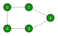
Example: Input: Graph:
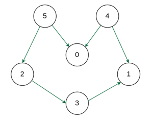
- Output: 5 4 2 3 1 0
- Explanation: The first vertex in topological sorting is always a vertex with an in-degree of 0 (a vertex with no incoming edges).
- A topological sorting of the following graph is: “5 4 2 3 1 0”.
- There can be more than one topological sorting for a graph.
- Another topological sorting of the following graph is: “4 5 2 3 1 0”.
Graph Algorithms Overview
Warshall's Algorithm
Warshall's Algorithm: A dynamic programming algorithm used to find the transitive closure of a directed graph.
In simpler terms, it determines whether there exists a path between every pair of vertices in the graph. It efficiently calculates the reachability matrix, which indicates whether a vertex can be reached from another vertex in the graph.
Dijkstra's Algorithm
Dijkstra's Algorithm: A greedy algorithm used to find the shortest path between a source node and all other nodes in a weighted graph.
It works by iteratively selecting the unvisited node with the smallest tentative distance from the source node, and then updating the distances of its neighbors. This process continues until all nodes have been visited.
Prim's Algorithm
Prim's Algorithm: A greedy algorithm used to find the Minimum Spanning Tree (MST) of a connected, weighted, undirected graph.
It starts with an initial vertex and iteratively adds the edge with the minimum weight that connects a vertex in the MST to a vertex outside the MST. This process continues until all vertices are included in the MST.
Kruskal's Algorithm
Kruskal's Algorithm: Another greedy algorithm used to find the MST of a connected, weighted, undirected graph.
It sorts all edges in non-decreasing order of their weight and iteratively adds the edge with the minimum weight that doesn't create a cycle in the MST. This process continues until all vertices are connected.
Minimum Spanning Trees
Introduction to Minimum Spanning Trees:
A minimum spanning tree (MST) or minimum weight spanning tree for a weighted, connected, undirected graph is a spanning tree with a weight less than or equal to the weight of every other spanning tree.
Introduction to Kruskal’s Algorithm:
Here we will discuss Kruskal’s algorithm to find the MST of a given weighted graph.
In Kruskal’s algorithm, sort all edges of the given graph in increasing order. Then it keeps on adding new edges and nodes in the MST if the newly added edge does not form a cycle.
It picks the minimum weighted edge at first and the maximum weighted edge at last. Thus we can say that it makes a locally optimal choice in each step in order to find the optimal solution. Hence this is a Greedy Algorithm.
How to find MST using Kruskal’s algorithm?
- Sort all the edges in non-decreasing order of their weight.
- Pick the smallest edge. Check if it forms a cycle with the spanning tree formed so far. If the cycle is not formed, include this edge. Else, discard it.
- Repeat step#2 until there are (V-1) edges in the spanning tree.
Step 2 uses the Union-Find algorithm to detect cycles.
Kruskal’s algorithm to find the minimum cost spanning tree uses the greedy approach. The Greedy Choice is to pick the smallest weight edge that does not cause a cycle in the MST constructed so far.
Illustration:
Below is the illustration of the above approach:
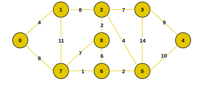
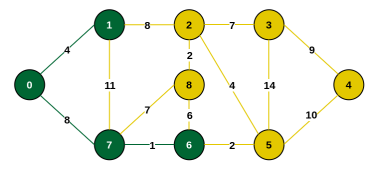
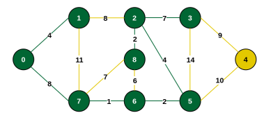
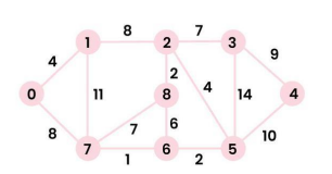
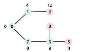
Input Graph:
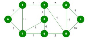
The Graph Analysis
The graph contains 9 vertices and 14 edges. So, the minimum spanning tree formed will be having (9 – 1) = 8 edges.
After Sorting:
| Weight | Source | Destination |
|---|---|---|
| 1 | 7 | 6 |
| 2 | 8 | 2 |
| 2 | 6 | 5 |
| 4 | 0 | 1 |
| 4 | 2 | 5 |
| 6 | 8 | 6 |
| 7 | 2 | 3 |
| 7 | 7 | 8 |
| 8 | 0 | 7 |
| 8 | 1 | 2 |
| 9 | 3 | 4 |
| 10 | 5 | 4 |
| 11 | 1 | 7 |
| 14 | 3 | 5 |
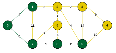
Step-by-Step Execution:
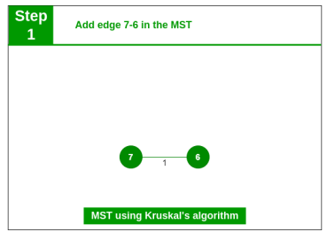
Step 1: Pick edge 7-6. No cycle is formed, include it.
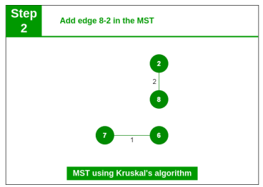
Step 2: Pick edge 8-2. No cycle is formed, include it.
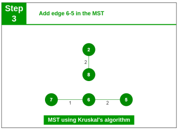
Step 3: Pick edge 6-5. No cycle is formed, include it.
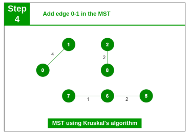
Step 4: Pick edge 0-1. No cycle is formed, include it.
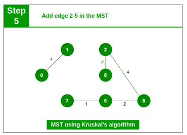
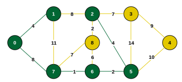
Step 5: Pick edge 2-5. No cycle is formed, include it.
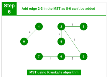
Step 6: Pick edge 8-6. Cycle formed, discard it. Pick edge 2-3. No cycle is formed, include it.
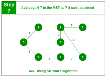
Step 7: Pick edge 7-8. Cycle formed, discard it. Pick edge 0-7. No cycle is formed, include it.
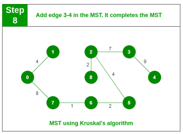
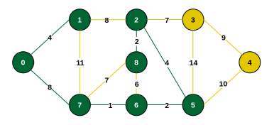
Step 8: Pick edge 1-2. Cycle formed, discard it. Pick edge 3-4. No cycle is formed, include it. Since we now have (9-1)=8 edges, the algorithm stops.
Prim’s Algorithm
Like Kruskal’s algorithm, Prim’s algorithm is also a Greedy algorithm. This algorithm always starts with a single node and moves through several adjacent nodes, in order to explore all of the connected edges along the way.
The algorithm starts with an empty spanning tree. The idea is to maintain two sets of vertices. The first set contains the vertices already included in the MST, and the other set contains the vertices not yet included. At every step, it considers all the edges that connect the two sets and picks the minimum weight edge from these edges. After picking the edge, it moves the other endpoint of the edge to the set containing MST.
How does Prim’s Algorithm Work?
- Step 1: Determine an arbitrary vertex as the starting vertex of the MST.
- Step 2: Follow steps 3 to 5 till there are vertices that are not included in the MST (known as fringe vertex).
- Step 3: Find edges connecting any tree vertex with the fringe vertices.
- Step 4: Find the minimum among these edges.
- Step 5: Add the chosen edge to the MST if it does not form any cycle.
- Step 6: Return the MST and exit.
Illustration of Prim’s Algorithm:
Consider the following graph as an example for which we need to find the Minimum Spanning Tree (MST).
Step 1: Select vertex 0 as the starting vertex.
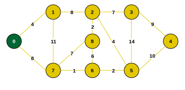
Step 2: The edges connecting the tree to other vertices are {0, 1} and {0, 7}. The minimum is {0, 1}. Include vertex 1.
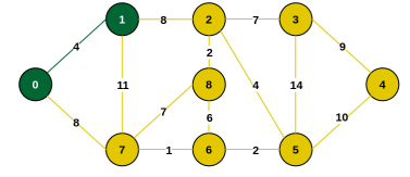
Step 3: Connecting edges are {0, 7}, {1, 7}, {1, 2}. Minimum is 8 for {0, 7} and {1, 2}. Choose {0, 7}. Include vertex 7.
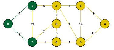
Step 4: Connecting edges are {1, 2}, {7, 6}, {7, 8}. Minimum is {7, 6} (weight 1). Include vertex 6.
Step 5: Connecting edges are {7, 8}, {1, 2}, {6, 8}, {6, 5}. Minimum is {6, 5} (weight 2). Include vertex 5.
Step 6: Minimum connecting edge is {5, 2} (weight 4). Include vertex 2.
Step 7: Minimum connecting edge is {2, 8} (weight 2). Include vertex 8.
Step 8: Minimum connecting edge is {2, 3} (weight 7). Include vertex 3.
Step 9: Minimum connecting edge is {3, 4} (weight 9). Include vertex 4.
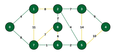
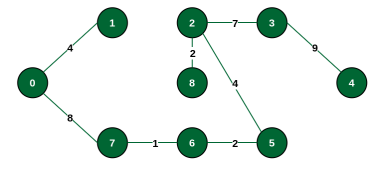
The final MST has a total weight of 37.
Shortest Paths from Source to all Vertices
Dijkstra’s Algorithm
Given a weighted graph and a source vertex in the graph, find the shortest paths from the source to all the other vertices in the given graph (with no negative edge weights).
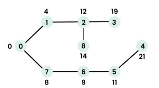
Example with src = 0:
Output Distances: 0 4 12 19 21 11 9 8 14
Algorithm:
- Create a set `sptSet` (shortest path tree set) to track finalized vertices. Initially empty.
- Assign distance values to all vertices: 0 for the source, INFINITE for all others.
- While `sptSet` doesn’t include all vertices:
- Pick a vertex `u` not in `sptSet` with the minimum distance value.
- Include `u` in `sptSet`.
- Update distance values of all adjacent vertices of `u`. For an adjacent vertex `v`, if `distance(u) + weight(u,v) < distance(v)`, then update `distance(v)`.
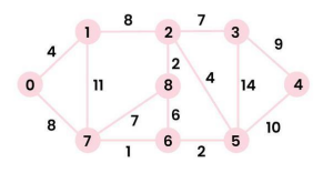
Illustration of Dijkstra Algorithm:
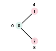
Considering the graph below with src = 0.
Step 1: `sptSet` = {0}. Distances updated for neighbors 1 (to 4) and 7 (to 8).
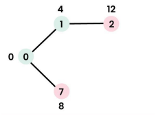
Step 2: Pick vertex 1. `sptSet` = {0, 1}. Update distance for neighbor 2 (to 4+8=12).
Step 3: Pick vertex 7. `sptSet` = {0, 1, 7}. Update distances for neighbors 6 (to 8+1=9) and 8 (to 8+7=15).
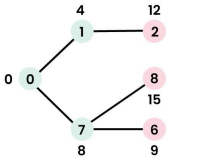
Step 4: Pick vertex 6. `sptSet` = {0, 1, 7, 6}. Update distances for neighbors 5 (to 9+2=11) and 8 (9+6=15, no change).
The process continues until all vertices are in `sptSet`, resulting in the final shortest path tree.
Transitive closure of a graph using Floyd Warshall Algorithm
Given a directed graph, determine if a vertex j is reachable from another vertex i for all vertex pairs (i, j). This reachability matrix is called the transitive closure.
For example, consider the graph below:
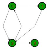
The Floyd Warshall Algorithm can be adapted to solve this. Instead of storing path lengths, we can store a boolean value indicating reachability. The core idea is to iterate through all vertices `k` and for every pair `(i, j)`, update the reachability `reach[i][j]` as `reach[i][j] || (reach[i][k] && reach[k][j])`.